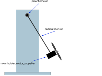
AEROPENDULUM PROJECT
Eniko T. Enikov, Associate Professor, University of Arizona
in collaboration and with the support of Giampiero Campa, Technical Evangelist, Mathworks Inc.
 2011 2012
Contents
- Installation Instructions
- The Aeropendulum Target Board
- Mathematical Model
- Open Loop Step Response
- Initial Parameter Identification
- Model Correction and Feedback Linearization
- Weightless Pendulum (Type 1 system)
- System Identification
- Design of Dynamic Compensator: Lag Compensator
- Design of Dynamic Compensator: Lead Compensator
- Advanced Studies: State-Space Controller and Observer Design
- Further Studies
- Pendulum Order Form, Inquiries, and Related Links
Installation Instructions
Assemble the pendulum according to the video instructions provided on the following Youtube Channel. (Instructions in other languages are also available.)
The Aeropendulum is powered by the USB port. It also communicates with MATLAB through a generic USB to Serial driver which comes with the Windows operating system. The target board operates on 32-bit and 64-bit systems, however at this time, only 32-bit versions of Matlab support external mode of Real Time Workshop. To cirucument this limitation, we have developed a new version of the Aeropendulum control interface (AeropendulumSoft.mdl), which operates in "soft" real-time mode with the help of an additional m-function (ms_fun_realtime_pacer.m). This function needs to be present in the Matlab working directory where the AeropendulumSOFT.mdl resides.
The installation process includes the following steps:
- Download and save the USB driver (32- or 64-bit version) from the following links USB_Driver32.inf or USB_Driver64.inf to a known location on your computer, e.g. Desktop, etc. (Use Right-Click and Save Link As... option.)
- For older systems (Win XP) - connect the target board to the USB port. The operating system will ask you for a driver location - browse to the directory where you saved the USB_Driver.inf file. The installation process should recognize this file and complete the driver installation. If a message appears about the fact that the driver has not passed the "windows logo testing", click on "Continue Anyway". When ready, you can check the successful installation by opening the Device Manager in the Control Panel and verifying that a COM port is associated with the pendulum. Typically this is COM4 or COM5. If the number of the associated COM port is greater than 8, it is suggested to force the port to an (unused) port between COM1 and COM8. This can be done from the Device Manager by double clicking on the "AMNL USB Serial Communication" port, accessing the "Port Settings" tab, clicking on the "Advanced" button, and selecting the desired port number.
- For newer systems (Vista, Win7) the installation require an additional disk clean-up step, that removes temporary files. Prior to connecting the pendulum, you need to perform manual disk clean up. When connecting the pendulum, the installation initially will result in an error, and you will need to manually point the installer to the location of your .inf file. If you do not perform disk clean properly, the installation will report a "Code 10" error. To perform this step, follow a detailed step-by-step instructions described on the following link Installation.pdf
- Start MATLAB and acivate the Real Time Windows Target Environment by issuing rtwintgt -setup in the command prompt.
- For 32-bit systems operating with true Real Time Windows Target, download a the Aeropendulum.mdl and Controllers.mat files from the website and save them in your MATLAB's working directory. (Use Right-Click and Save Link As... option.) Load the Controllers.mat file by issuing the command load Controllers This step will pre-load variables clagd and clead which are z-domain models of the lag and lead controllers. The Aeropendulum.mdl looks for these varaiables and therefore will only compile when they exist in the workspace. Open the Aeropendulum.mdl file and re-compile. This can be done from the "tools" menu, selecting "Code Generation" and then "Build Model", by jointly clicking the "CTRL" and "B" keys when the model is selected, or typing "rtwbuild('Aeropendulum')" from the command line. If there are no errors, connect to target and run. If there are errors connecting, check the values of the COM ports in the Packet Input and Packet Outpu blocks. They need to match the port associated with the USB to Serial driver. See the step on how to install the board to make sure you know to which COM port the pendulum is connected to. The provided Aeropedulum.mdl file uses a default value of COM4 in its Packet Input and Packet Output blocks. If your pendulum is installed on a different COM port, you need to update these blocks by opening the Pendulum I/O (plant) group and updating (associating) the COM port settings in the Packet Ouput and Packet Input blocks. There are a total of three such blocks. Two of them are located in the Query Instrument group and one is immediately visible inside the Pendulum I/O group. Make sure all of them match the COM port associated with your pendulum. When all these updates have been completed, you should be able to re-compile the Aeropendulum.mdl model and connect it to taget by using the Connect to Target button. To run it, you need to click on Play button. The pendulum should run for 60 seconds.
- For newer 64-bit systems operating in soft-real time, download the .mdl file from AeropendulumSOFT.mdl and msfun_realtime_pacer.m and save them in the same working directory. The COM port settings, as well as initial values of controller transfer functions are defined in the "model properties" block under the "File" menu. More specifically, these can be found in the "Call-Back" menu. Therefore, after downloading and saving the .mdl file, you only need to update the call back options as described in Installation.pdf This version of the controller does not require compilation and you can run it as conventional simulink file by pressing the play button. The drawback of using soft real-time mode is that depending the performance of your system, the update rate might be too slow and with interuptions. Newer systems are generally fast enough and can produce 100 ms sampling time.
- When using true real-time, you can make changes to the controller selecting switch without re-compiling. Also you can change the value of the parameters and PWM values without re-compiling. However, if you modify the transfer functions clagd and clead, you do need to re-compile. When using soft real-time, you do not need to re-compile but some changes to the model while running, might interfere and interupt the operation of the aeropendulum.
The Aeropendulum Target Board
The target board is programmed to respond to commands from the PC. It always receives one byte and depending on its value either sends a PWM command to the motor or returns the voltage of the potentiometer in two bytes (12 bit conversion). For each cycle, MATLAB sends a signed integer. The values from -127 to 127 are converted into a PWM singal from -100% (negative direction) to +100% - positive direction of rotation. The value of -128 is reserved as the command for reading the potentiometer and sending two bytes containing the 12-bits of the ADC result. Since the "Packet Out" block codes integers using two's complement, and wraps around its range, if N is the value at the block input, the value that is sent via serial port is mod(128+N,256)-128. So for example values in from 128 to 255 are mapped in the range from -128 to -1. Therefore, except for the open loop module, all other controllers have a saturation block forcing the control signal to be in the [-127, 127] range.
Mathematical Model
We start by developing a mathematical model of the pendulum:

where  is the displacement angle, L is the pendulum length and
  is the input voltage to the motor. In reality, instead of controlling the voltage, the target board generates a pulse-width modulated (PWM) signal with amplitude of 5 V and a varying duty cycle, which is sent to the motor. Therefore in all subsequent discussions will denote the value of PWM signal. The coefficient
  denotes the conversion of the the PWM signal into a thrust force. This is only an approximate model as this thrust depends also on the relative velocty of the air and hence on the rate of swinging of the pendulum
  . For the purposes of this project, these effects are neglected.
Open Loop Step Response
After activating the Real Time Windows Target environment (one-time activation is sufficient for all subsequent sessions of MATLAB), open the Aeropendulum model
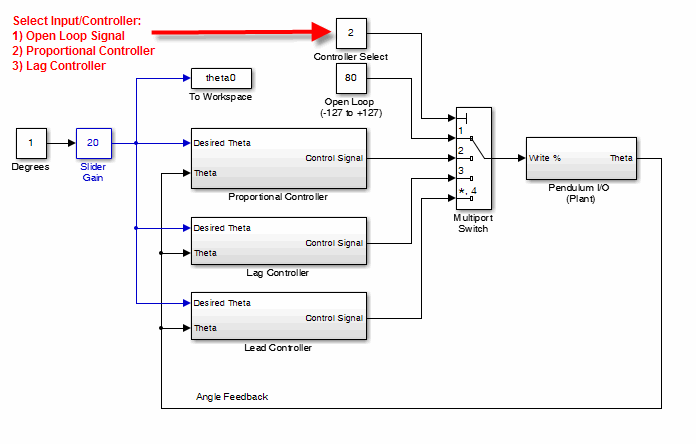
Enter the value 1 in the Control select block and a value between -127 and 127 in the Open Loop source block. Click on the "connect to target" button and run the model. The output angle should be visible in the Scope window. Four signals are exported to the workspace for further processing: (1) the time vector  ; the input reference angle
  ; the output angle ; and the PWM signal sent to the target
  . In command mode you can plot and examine these signals
%plot(t,theta)
%xlabel('Time, sec')
%ylabel('Ouput angle, deg')
Initial Parameter Identification
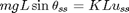
By examining the steady-state behaviour of the system model, it is apparent that we can determine some of the model parameters by running a series of open-loop response tests. Notice that at steady-state, sine of the ouput angle and the input PWM signal follow a linear relationship:
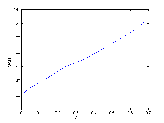
Run several experiments by choosing different values of the PWM signal between 0 and 127 and gather the steady-state output angles
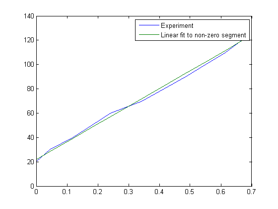
u_ss=[0 10 20 30 40 50 60 70 80 90 100 110 120 127];
theta_ss=[0 0 0 2.5 6.8 10.5 14 20 24.5  29.  33.4 38  42 43];
sine_ss=sind(theta_ss);
figure
plot(sine_ss,u_ss)
ylabel('PWM Input')
xlabel('SIN theta_{ss}')
- Can you repeat this for negative values of the input PWM?
- Do you expect a symmetric response?
- If there are any differences, what could be their physical explanation?
As can be seen, the system has a dead-band, i.e. for small PWM values, the pendulum does not move. The resutling linear curve has a horizonal offset of  and a slope of
  , which are the first two parameters of the model. To estimate them, we use linear curve fitting
figure
P=polyfit(sine_ss(3:14),u_ss(3:14),1)
plot(sine_ss,u_ss,sine_ss(3:14), polyval(P,sine_ss(3:14)))
shg
legend('Experiment','Linear fit to non-zero segment')
P =

  145.8891   21.9263
Update the Design Parameters block of Aeropendulum.mdl model by entering the values of the parameter  and
and  found from the above curve fitting.
Model Correction and Feedback Linearization
With the parameters  and determined, it is now possible to correct the model so that it captures the fact that the pendulum does not move until the input exceeds the value Specifically, for positive values of the input we have:

It is now possible to re-define the control signal such that the nonlinear term  and the dead-band cancel out. Notice that, assuming
  if we introduce:
the model becomes linear:
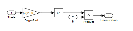
Open any of the controller blocks to find the implementation of the feedback linearization in Simulink
Weightless Pendulum (Type 1 system)
In controls terminology, the feedback-linearized open-loop transfer function represents a second-order system of Type 1, i.e. it has an integrator (a pole at the origin). Therefore, if a zero input is presented to it, the output will remain constant, i.e. the pendulum will self-balance itself at any angle. This condition can be used to verify the correct values of the parameters and  . To check this, select input = 2 (proportional controller) and enter a value 0 for the proportional gain
  . Run the model. If the pendulm is balanced, you should be able to move it with your hand and leave it at random positions as shown by the flat portions of the output and PWM signals below
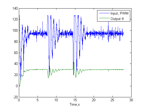
load KP0Response
figure
plot(t,PWM,t,theta)
legend('Input, PWM','Output \theta')
xlabel('Time,s')
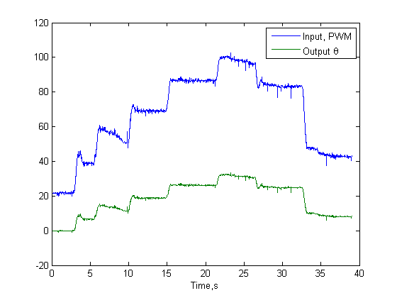
If for some reason your pendulum drops or keeps going up, that means that the either or is too low or too high, respectively.
- Can you tell which parameter needs adjustment by observing the behaviour of the pendulum at small and larger angles?
System Identification
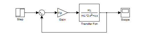
The block diagram of the feedback-linearized pendulum model is shown below:
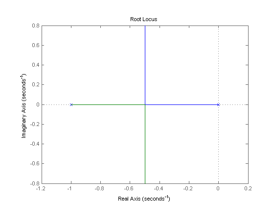
where the two poles are at 0 and  . The root locus of a similar system with a pole at 0 and -1 is shown below
g=tf(1,[1 1 0])
rlocus(g)
g =

     1
  -------
  s^2 + s

Continuous-time transfer function.
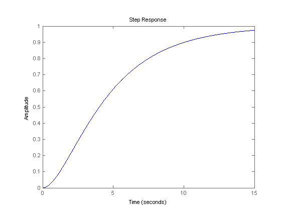
For low values of the gain Kp (say Kp=0.1), the system is overdamped and its step response shows no overshoot. Essentially, the system behaves as two first-order systems connected in series
step(0.2*g/(1+0.2*g),[0:0.01:15])
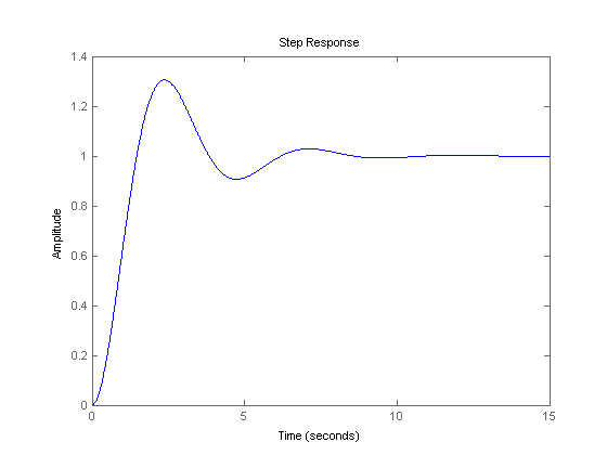
For higher value of the gain Kp (say Kp=2), the sytems is underdamped and its step response shows increasinlgy larger overshoot.
step(2*g/(1+2*g),[0:0.01:15])
Run the Aeropendulum model for various values of the gain ranging from 0.1 to 2.5 and observe the response.
- What is the behaviour of the Aeropendulum for
 (under/overdemped)?
- What is the behavior of the Aeropendulum for
 (under/overdamped) ?
If accurately feedback-linearized, the pendulum will be overdamped) for  , and underdamped for
  . Let's indentify its parameters using MATLAB System Identification Toolbox using the
  experiment.
Set the reference input  and and run the experiment. The respone of the unit-feedback system should be available in the workspace. You need about 10 seconds worth of data.
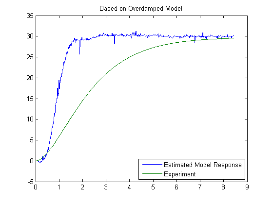
load KP1Response
% Create a data object to be used for system identification
DAT = iddata(theta,theta0,0.01);
% Use 'p2' for two overdamped poles,
% 'p2u' for a system with two underdamped poles
% Extract a predicion-estimate model of the system using
% the assumed form of overdamped system
m1 = pem(DAT,'p2')
% Convert the model to state space description CL
CL=idss(m1);
% Convert state space description to transfer function
[n1 d1]=ss2tf(CL.A,CL.B,CL.C,CL.D,1)
% Ingore n1(1) and n1(2) due to being very small
gCL=tf(n1(3),d1)
% Simulate response from the model and compare with experiment
[y1,t1]=lsim(gCL,theta0,t);
figure
plot(t,theta,t1,y1)
legend('Estimated Model Response','Experiment','location','SouthEast')
title('Based on Overdamped Model')
Warning: There is an indication of underdamped modes in the model.
Consider including a "U" string in the "Type" value when generating
the model.

m1 =
Process model with transfer function:
                 Kp
G(s) = ------------------
          (1+Tp1*s)(1+Tp2*s)


       Kp = 0.98609
      Tp1 = 0.47209
      Tp2 = 0.47207

Parameterization:
    'P2'

   Number of free coefficients: 3
   Use "getpvec", "getcov" for parameters and their uncertainties.

Status:
Estimated using PROCEST on time domain data "DAT".
Fit to estimation data: 80.7% (prediction focus)
FPE: 4.116, MSE: 2.617

n1 =

         0         0    4.4247


d1 =

    1.0000    4.2366    4.4871


gCL =

          4.425
  ---------------------
  s^2 + 4.237 s + 4.487

Continuous-time transfer function.
Now let's try to estimate the system assuming it is underdamped
m1 = pem(DAT,'p2u')
CL=idss(m1);
[n1 d1]=ss2tf(CL.A,CL.B,CL.C,CL.D,1)
gCL=tf(n1(3),d1)
[y1,t1]=lsim(gCL,theta0,t);
figure
plot(t,theta,t1,y1)
legend('Estimated Model Response','Experiment','location','SouthEast')
title('Based on Underdamped Model')
m1 =
Process model with transfer function:
                   Kp
G(s) = ----------------------
          1+2*Zeta*Tw*s+(Tw*s)^2


       Kp = 0.99938
       Tw = 0.43321
     Zeta = 0.79015

Parameterization:
    'P2U'

   Number of free coefficients: 3
   Use "getpvec", "getcov" for parameters and their uncertainties.

Status:
Estimated using PROCEST on time domain data "DAT".
Fit to estimation data: 91.84% (prediction focus)
FPE: 0.473, MSE: 0.468

n1 =

         0         0    5.3251


d1 =

    1.0000    3.6479    5.3285


gCL =

          5.325
  ---------------------
  s^2 + 3.648 s + 5.328

Continuous-time transfer function.
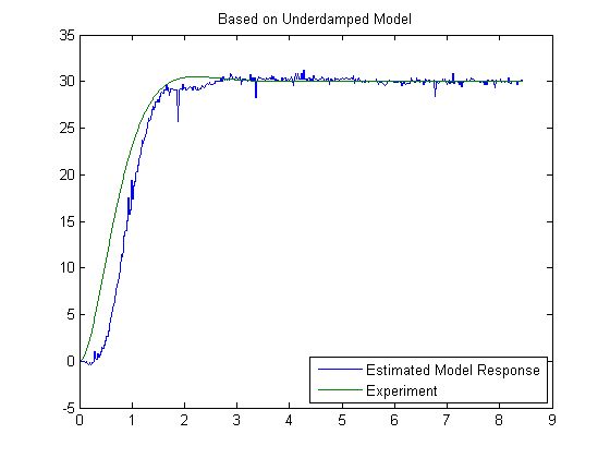
A much better agreement is obtained using the underdampced model with large damping, altough there are still noticeble differences.
- What could be a possible cause of these discrepancies? (Hint: Run the pendulum for
 and observe the change in the behavior of the system. Does it remain stable for large values of
  ? What do we know about the stablity of a second order system based on its root locus for large values of the gain? Is this true for a higher oder systems with no zeros? Below is a plot of the response for
  .
.
load KP3Response
figure
plot(t,theta,t,PWM)
legend('\theta','PWM','location','SouthEast')
%
%  Based on the observed differences between expected stabiltiy and the
%  response of the system we conclude that the system must be of higher
%  order. Nevertheless, we can design a dynamic compenstator based on the
%  imperfect model derived so far.
Design of Dynamic Compensator: Lag Compensator
Using the derived model gCL, one can obtain the open loop transfer
function using a positive feeback.
- Prove that a positive unit feedback around a negative feedback returns the open loop transfer function.
gOL=feedback(gCL,1,+1)
gOL =

           5.325
  ------------------------
  s^2 + 3.648 s + 0.003326

Continuous-time transfer function.
Notice the small value of the constant term of the denominator. For a type 1 system this term should be zero. The reason for a non-zero, but small value is the fact that the feedback linearization is not perfect, i.e. the gravitational force is not fully compensated by the feedback.
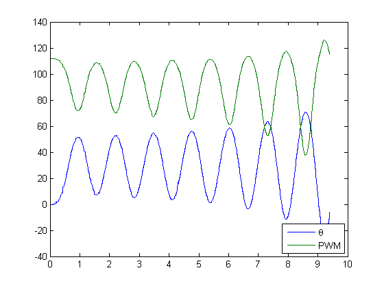
For the design of a dynamic compensator we can use the SISO tool. Use the following command to open SISOtool in "bode" mode in import the open loop transfer function.
sisotool('bode',gOL)
As evident, the system has 70 degrees of phase margin and will be stable under unit feedback.
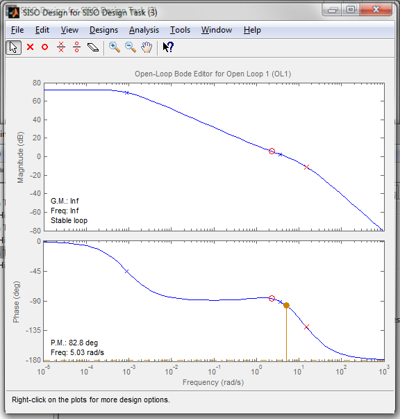
Using the SISOtool GUI, place a dominant pole at -0.06 , a zero at -0.48 and adjust the gain so that the gain cross-over frequency is 1. Export the compensator C to the workspace variable Clag and convert to a discrete transfer function using c2d
load Controllers
sisotool('bode',gOL,Clag,1,1)
Clag
clagd=c2d(Clag,0.01,'zoh')
Clag =

  0.82575 (s+0.4771)
  ------------------
     (s+0.05936)

Continuous-time zero/pole/gain model.


clagd =

  0.82575 (z-0.9952)
  ------------------
      (z-0.9994)

Sample time: 0.01 seconds
Discrete-time zero/pole/gain model.
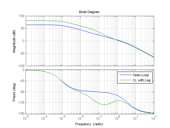
Examine the effect of the compensator by comparing Bode plots of the uncompensated and compenstated systems.
figure
bode(gOL,Clag*gOL)
legend('Open Loop','CL with Lag')
grid
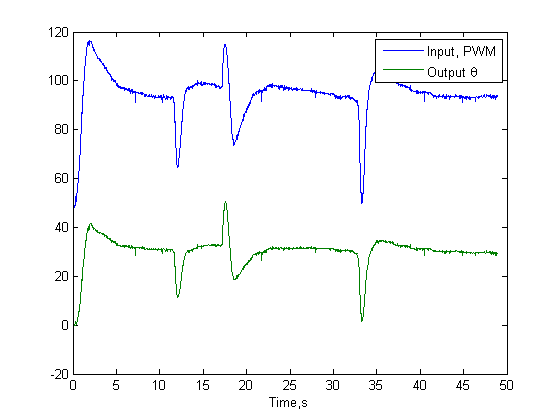
Run the Aeropendulum with input selector set to 3 to see the effect of the lag compensator.
load lagresponse
figure
plot(t,PWM,t,theta)
legend('Input, PWM','Output \theta')
xlabel('Time,s')
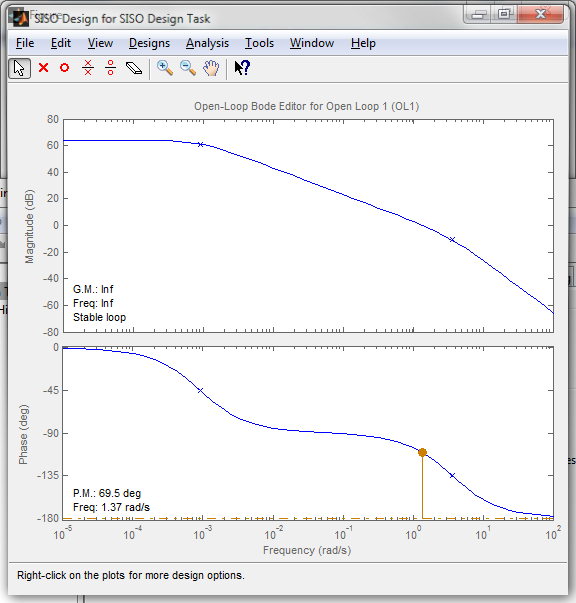
Design of Dynamic Compensator: Lead Compensator
Clear the SISOtool design by selecting Design->Clear->C Place a dominant zero at -2.33 and a less dominant pole at -15.23. Adjust the gain until the gain cross over frequency is at 5 rad/s. Export the model to Clead using the Export option and convert the continuous compensator into a discrete one
sisotool('bode',gOL,Clead,1,1)
clead=c2d(Clead,0.01,'zoh')
clead =

  16.979 (z-0.9784)
  -----------------
     (z-0.8587)

Sample time: 0.01 seconds
Discrete-time zero/pole/gain model.
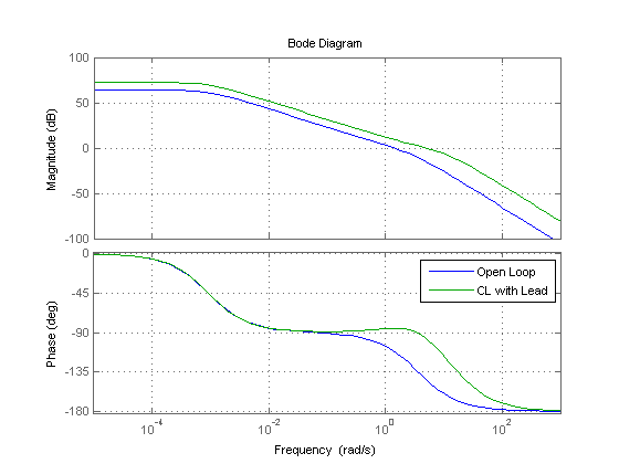
Examine the effect of the compensator by comparing Bode plots of the uncompensated and compenstated systems.
bode(gOL,Clead*gOL)
legend('Open Loop','CL with Lead')
grid
Run the Aeropendulum with input selector set to 3 to see the effect of the lag compensator.
load Leadresponse
figure
plot(t,PWM,t,theta)
legend('Input, PWM','Output \theta')
xlabel('Time,s')
Advanced Studies: State-Space Controller and Observer Design
Comming soon.
Further Studies
Through this example you have seen the use of system identification toolbox to extract a model of the system. As you might have noticed the overdamped second-order model did not fit well the experiment. While the underdamped version produced a better match, the fit was still not perfect. If you examine the discrepancies, you would notice that the difference occurs mainly at the beginning and the end of the step response. This pointts towards a faster dynamics that is not captured in the present model. The most obvious culprit is the propeller rotor dynamics, which in itself is a second order system. Therefore, one would expect that a fourth order model (two additional poles) would be required in order to better model the system.
- Repeat the system identificaiton step with a fourth order model and examine the level of agreement between model and experiment.
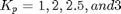
- Move the counterweight to the most extended position, so that the pendulum is self-balanced. Place the pendulum in a vertical starting position and command to move to a desired angle. You will notice that the previously design controllers do not work well. Turn off the feedback linearization, since it is now provided by the counterweight. Design a controller that moves the pendulum forward with 40
 PWM if the error is positive and -80 PWM if the error is negative. This is so-called bang-bang or on/off controller. An example of the operation is shown below.
Pendulum Order Form, Inquiries, and Related Links
Pendululum kits can be purchased by filling out the following Order Form and faxing it to +1(520)621-2236.
Additional Resources:
- Instructors can make request for sample files used in these demonstrations via email to enikov@email.arizona.edu
- IEEE Transactions on Education 2012:Mechatronic Aeropendulum: Demonstration of Linear and Non-Linear Feedback Control Principles with Matlab/Simulink Real-Time Windows Target